GUI
Using the GUI
Note: the GUI requires panel and bokeh to
be available in the current environment.
The Intake top-level singleton intake.gui gives access to a graphical data browser
within the Jupyter notebook. To expose it, simply enter it into a code cell (Jupyter
automatically display the last object in a code cell).
New instances of the GUI are also available by instantiating intake.interface.gui.GUI,
where you can specify a list of catalogs to initially include.
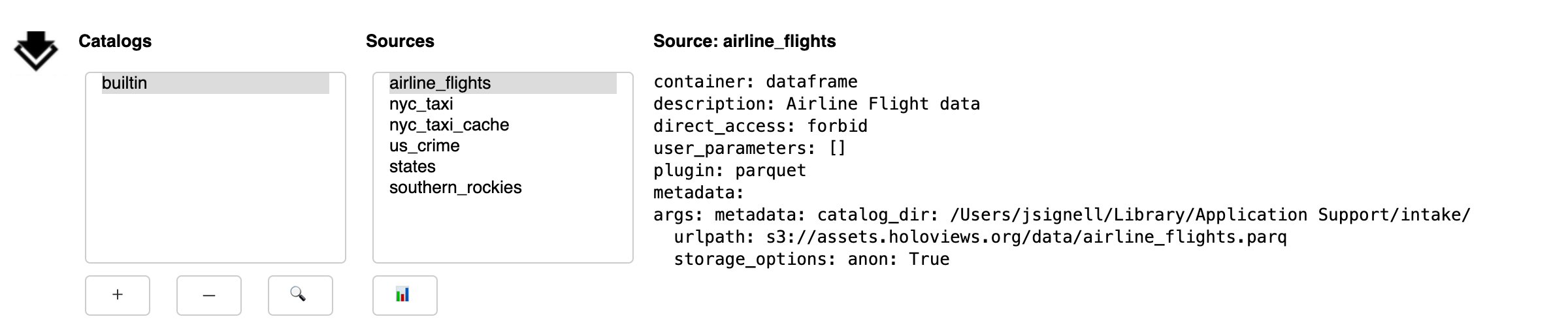
The GUI contains three main areas:
a list of catalogs. The “builtin” catalog, displayed by default, includes data-sets installed in the system, the same as
intake.cat.a list of sources within the currently selected catalog.
a description of the currently selected source.
Catalogs
Selecting a catalog from the list will display nested catalogs below the parent and display source entries from the catalog in the list of sources.
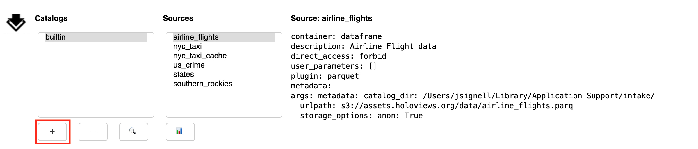
Below the lists of catalogs is a row of buttons that are used for adding, removing and searching-within catalogs:
Add: opens a sub-panel for adding catalogs to the interface, by either browsing for a local YAML file or by entering a URL for a catalog, which can be a remote file or Intake server
Remove: deletes the currently selected catalog from the list
Search: opens a sub-panel for finding entries in the currently selected catalog (and its sub-catalogs)
Add Catalogs
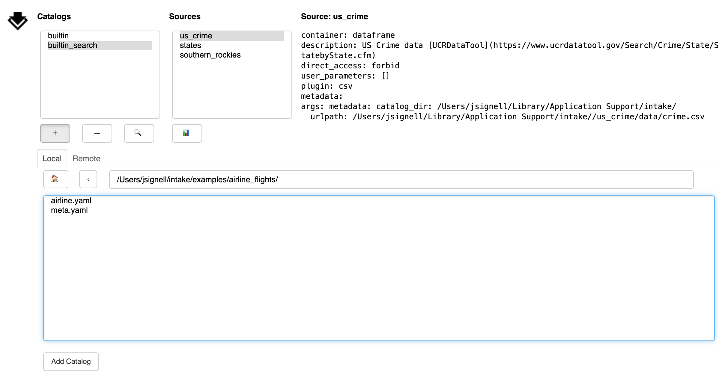
The Add button (+) exposes a sub-panel with two main ways to add catalogs to the interface:
This panel has a tab to load files from local; from that you can navigate around the filesystem using the arrow or by editing the path directly. Use the home button to get back to the starting place. Select the catalog file you need. Use the “Add Catalog” button to add the catalog to the list above.
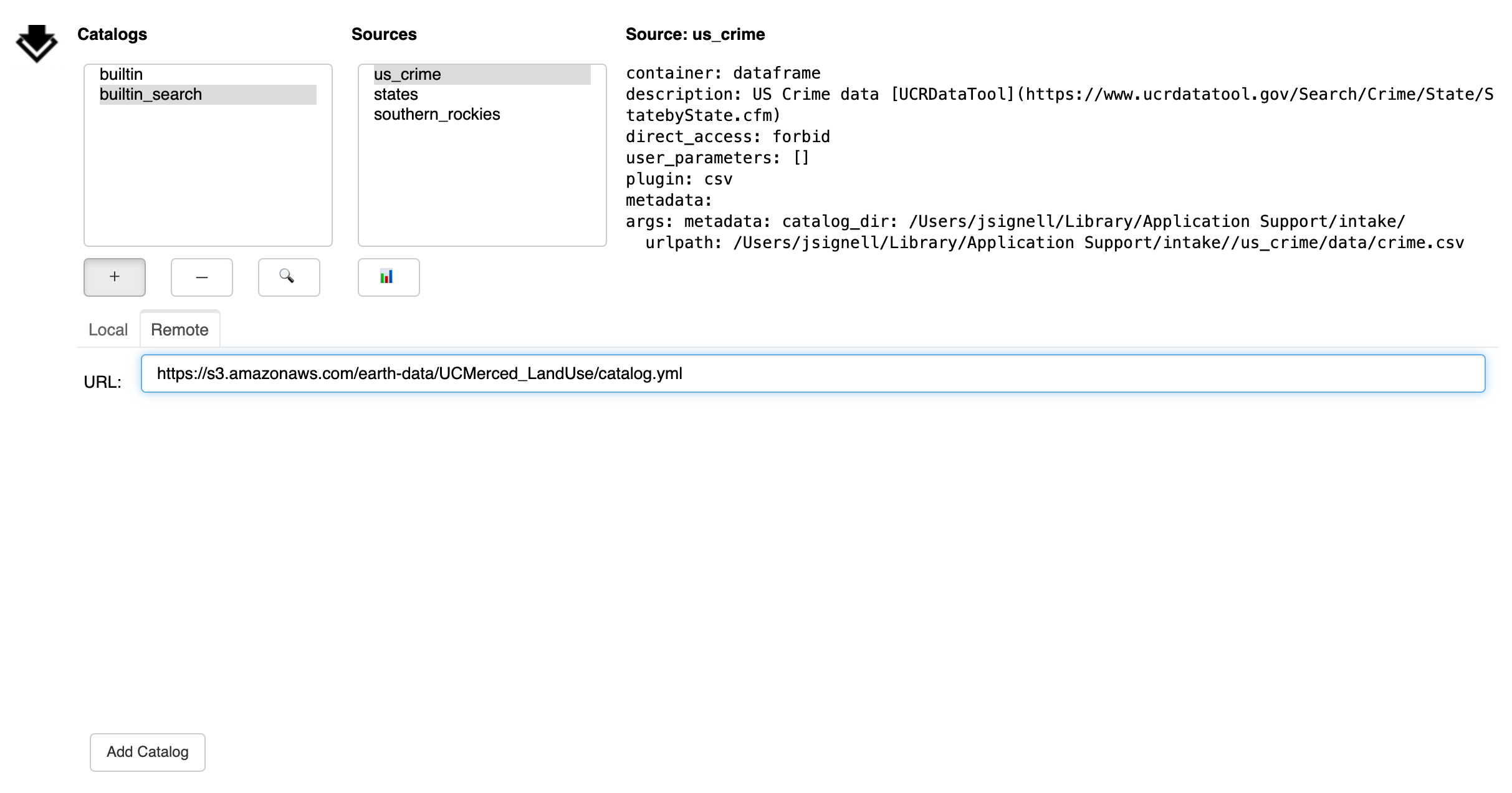
Another tab loads a catalog from remote. Any URL is valid here, including cloud locations,
"gcs://bucket/...", and intake servers, "intake://server:port". Without a protocol
specifier, this can be a local path. Again, use the “Add Catalog” button to add
the catalog to the list above.
Finally, you can add catalogs to the interface in code, using the .add() method,
which can take filenames, remote URLs or existing Catalog instances.
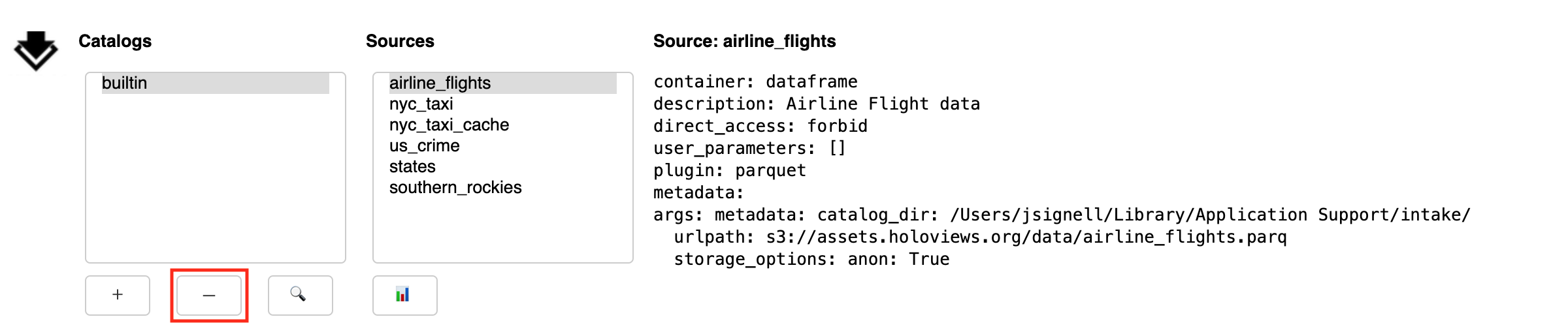
Remove Catalogs
The Remove button (-) deletes the currently selected catalog from the list. It is important to note that this action does not have any impact on files, it only affects what shows up in the list.
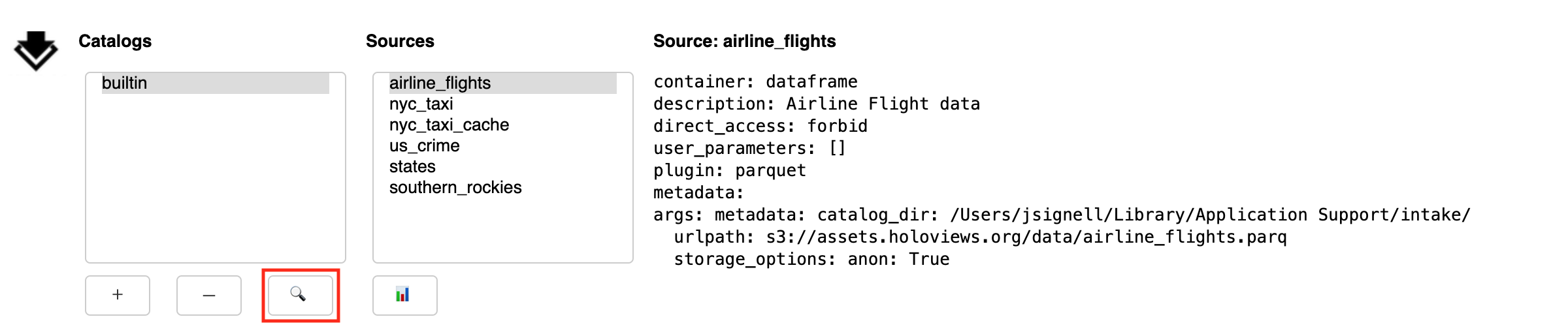
Search
The sub-panel opened by the Search button (🔍) allows the user to search within the selected catalog
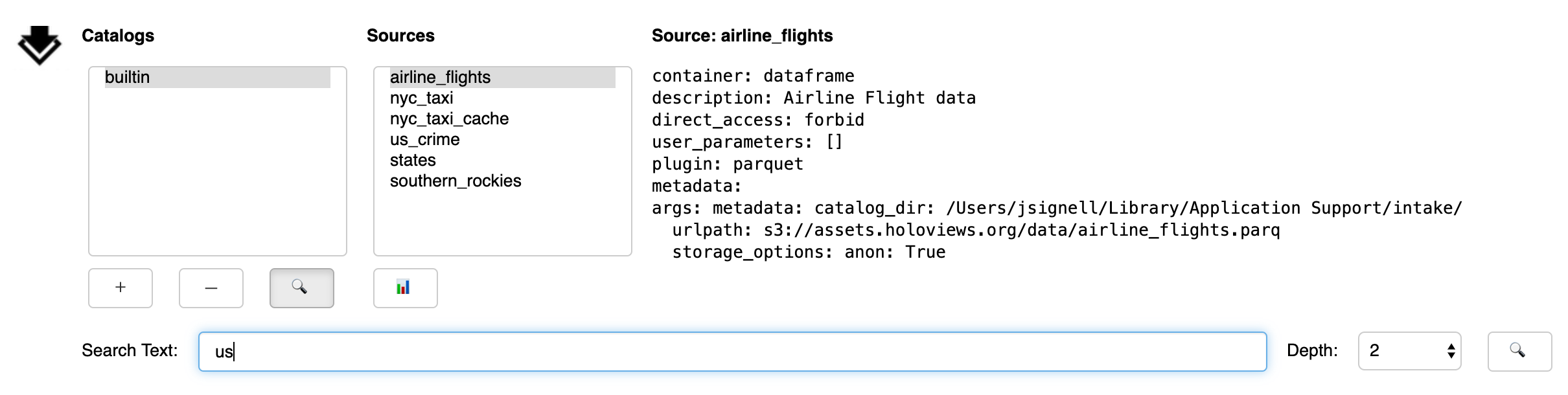
From the Search sub-panel the user enters for free-form text. Since some catalogs contain nested sub-catalogs, the Depth selector allows the search to be limited to the stated number of nesting levels. This may be necessary, since, in theory, catalogs can contain circular references, and therefore allow for infinite recursion.
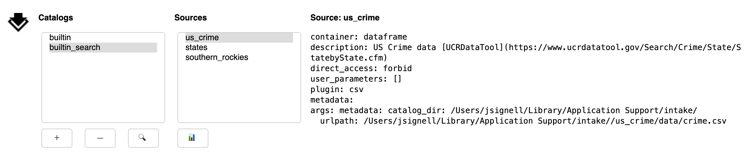
Upon execution of the search, the currently selected catalog will be searched. Entries will be considered to match if any of the entered words is found in the description of the entry (this is case-insensitive). If any matches are found, a new entry will be made in the catalog list, with the suffix “_search”.
Sources
Selecting a source from the list updates the description text on the left-side of the gui.
Below the list of sources is a row of buttons for inspecting the selected data source:
Plot: opens a sub-panel for viewing the pre-defined (specified in the yaml) plots for the selected source.
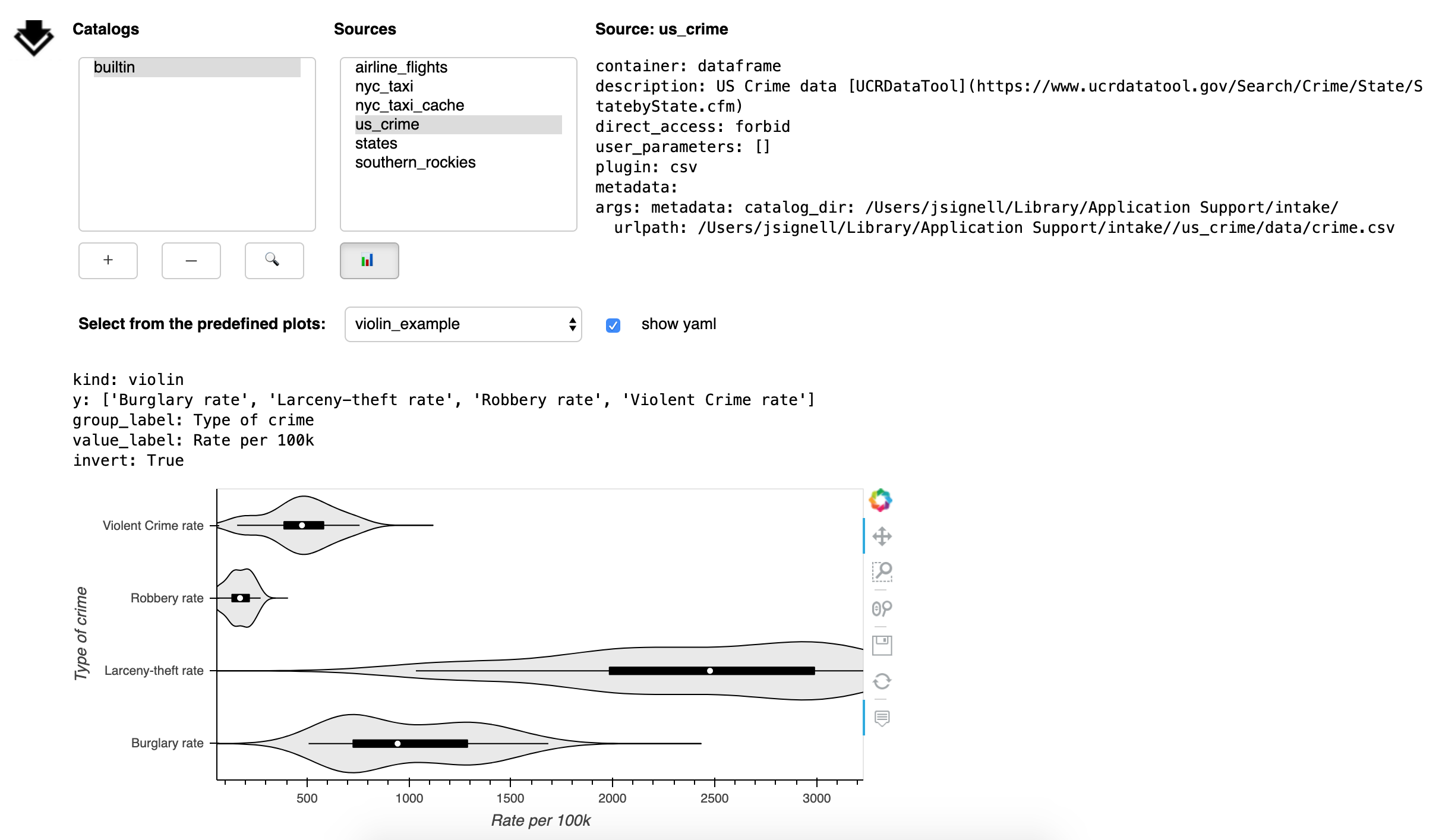
Plot
The Plot button (📊) opens a sub-panel with an area for viewing pre-defined plots.
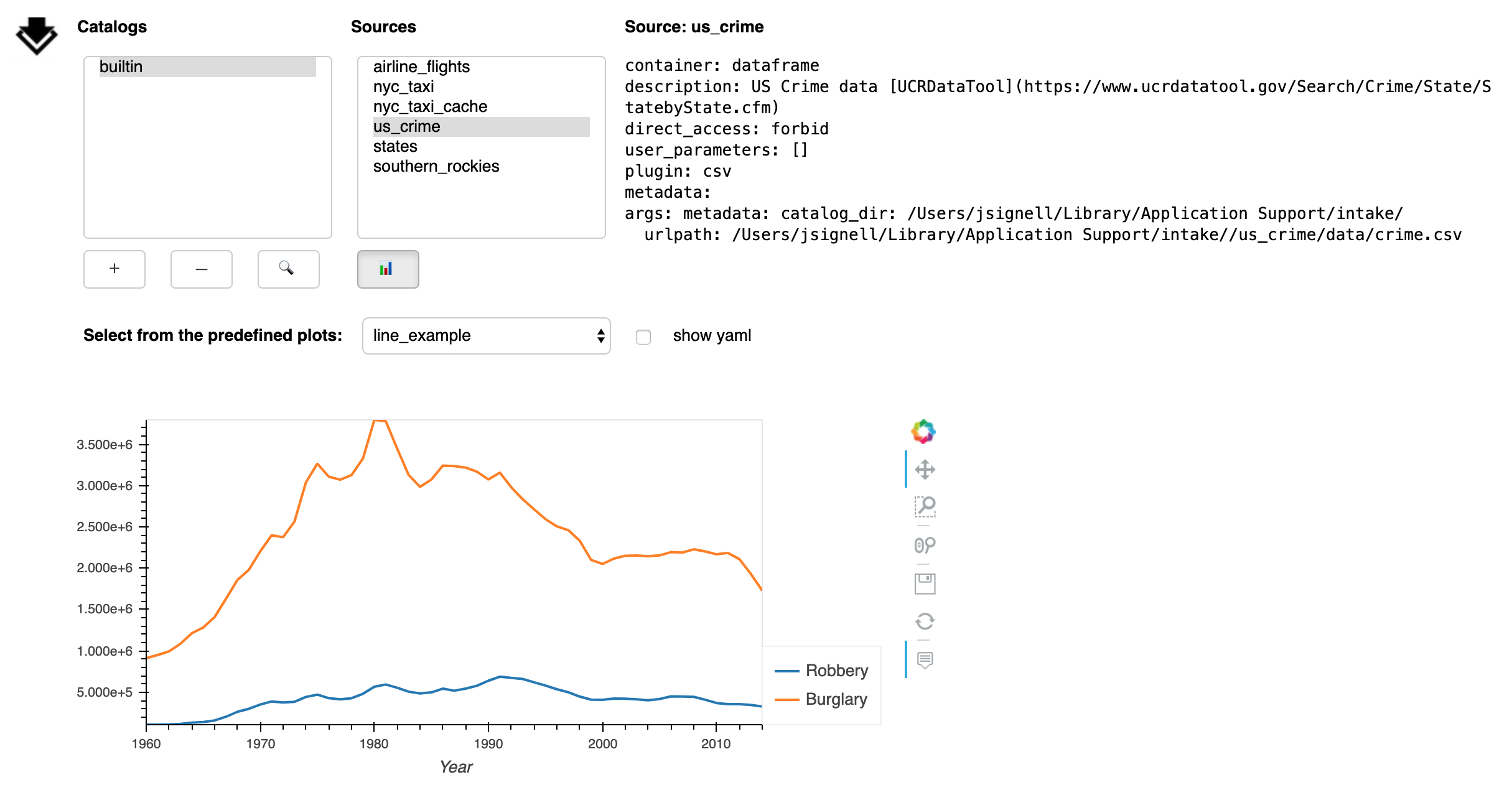
These plots are specified in the catalog yaml and that yaml can be displayed by checking the box next to “show yaml”.
The holoviews object can be retrieved from the gui using intake.interface.source.plot.pane.object,
and you can then use it in Python or export it to a file.
Interactive Visualization
If you have installed the optional extra packages dfviz and xrviz, you can interactively plot your dataframe or array data, respectively.
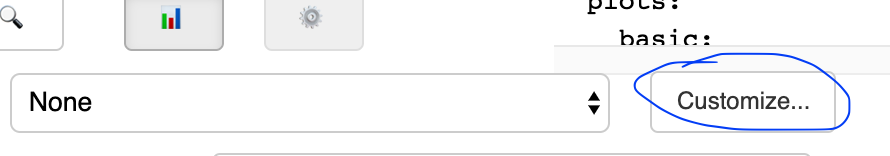
The button “customize” will be available for data sources of the appropriate type. Click this to open the interactive interface. If you have not selected a predefined plot (or there are none), then the interface will start without any prefilled values, but if you do first select a plot, then the interface will have its options pre-filled from the options
For specific instructions on how to use the interfaces (which can also be used independently of the Intake GUI), please navigate to the linked documentation.
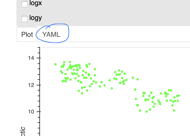
Note that the final parameters that are sent to hvPlot to produce the output
each time a plot if updated, are explicitly available in YAML format, so that
you can save the state as a “predefined plot” in the catalog. The same set of
parameters can also be used in code, with datasource.plot(...).
Using the Selection
Once catalogs are loaded and the desired sources has been identified and selected,
the selected sources will be available at the .sources attribute (intake.gui.sources).
Each source entry has informational methods available and can be opened as a data source,
as with any catalog entry:
In [ ]: source_entry = intake.gui.sources[0]
        source_entry
Out   :
name: sea_ice_origin
container: dataframe
plugin: ['csv']
description: Arctic/Antarctic Sea Ice
direct_access: forbid
user_parameters: []
metadata:
args:
  urlpath: https://timeseries.weebly.com/uploads/2/1/0/8/21086414/sea_ice.csv

In [ ]: data_source = source_entry()  # may specify parameters here
        data_source.read()
Out   : < some data >

In [ ]: source_entry.plot()  # or skip data source step
Out   : < graphics>